综述文章 CV中的注意力机制-2022

 文章原文：**Attention Mechanisms in Computer Vision: A Survey**

 本片中的方法代码实现Github，是基于新的框架Jittor

技术介绍

 注意力机制根据数据域分类。其中包含了四种分类：通道注意力、空间注意力、时间注意力、分支注意力，其中有两个重叠类，即通道-空间注意力(全体与局部结合)、空间-时间注意力(3D Conv中用到)。空集表示这种组合还不存在（2022年前）。

$$Attention=f(g(x),x)$$

 通道、空间和时间注意力能够被看作是在不同的域(维度)上操作。C表示通道域，H和W表示空间域，T表示时间域。分支注意力是对这些的补充。可以看作固定某几维后，按在剩余几维中点的重要性分配权重。

近期发展历程

1. 第一阶段：从RAM开始的开创性工作，将深度神经网络与注意力机制相结合。它反复预测重要区域。并以端到端的方式更新整个网络。之后，许多工作采用了相似的注意力策略。在这个阶段，RNN在注意力机制中是非常重要的工具。

2. 第二阶段：从STN中，引入了一个子网络来预测放射变换用于选择输入中的重要区域。明确预测待判别的输入特征是第二阶段的主要特征。DCN是这个阶段的代表性工作

3. 第三阶段：从SENet(Squeeze-and-Excitation Networks)开始，提出了通道注意力网络(channel-attention network)能自适应地预测潜在的关键特征。CBAM和ECANet是这个阶段具有代表性的工作

4. 第四阶段：self-attention自注意力机制。自注意力机制最早是在NLP中提出并广泛使用。Non-local Neural Networks网络是最早在CV中使用自注意力机制，并在视频理解和目标检测中取得成功。像EMANet，CCNet，HamNet和the Stand-Alone Network遵循此范式并提高了速度，质量和泛化能力。深度自注意力网络(visual transformers)出现，展现了基于attention-based模型的巨大潜力。

计算机视觉中的注意力机制

Symbol	Description	Translation
GAP	global average pooling	全局平均池化
GMP	global max pooling	全局最大池化
[]	concatenation	拼接（串联）
Expand	expan input by repetition	重复输入
δ	ReLU activation	ReLU激活函数
σ	sigmoid activation	sigmoid激活函数

D2L 注意力评分函数

任务	全称	缩写
分类	classification	Cls
检测	detection	Dec
语义分割	semantic segmentation	SSeg
实例分割	instance segmentation	ISeg
风格迁移	style transfer	ST
动作识别	action recognition	Action
细粒度分类	fine Grained Classification	FGCls
图片描述	image captioning	ICap
行人重识别	re-identification,	ReID
人体关键点检查	keypoint detection	KD

通道注意力(channel attention)

SENet

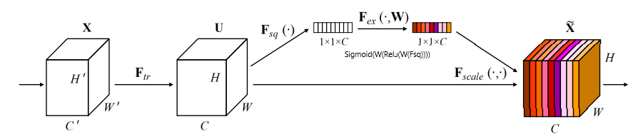
Squeeze-and-Excitation Networks

1. squeeze模块：全局平均池化(GAP)，压缩通道 [H,W][H,W]->[1,1][1,1]

2. excitation模块：后接全连接层($W_1$)->ReLU层($δ$)->全连接层($W_2$)->Sigmoid($σ$)

GSoP-Net

 Global Second-order Pooling Convolutional Networks

 改进： global average pooling(GAP) -> global second-order pooling(GSoP)

 $$Y = F_{gsop}(X, \theta) \cdot X = \sigma(W(RC(Cov(Conv(X))))) \cdot X$$

 $Cov$为协方差矩阵，$RC$为row-wise conv操作（不太懂）

 通过使用全局二阶池化(GSoP)，GSoPBlock提高了通过SEBlock收集全局信息的能力。然而，这是以额外计算为代价的。因此，通常在几个剩余块之后添加单个GSoPBlock

SRM

SRM : A Style-based Recalibration Module for Convolutional Neural Networks

$$Y = F_{srm}(X, \theta) \cdot X = \sigma(BN(CPC(SP(X)))) \cdot X$$

1. queeze模块：使用style pooling(SP)，它结合了全局平均池化和全局标准差池化。（为什么输出为 ${C\times{d}}$：当只用全局平均池化就是${C\times{1}}$；当用了全局平均池化和全局标准差池化就是${C\times{2}}$；当用了全局平均池化和全局标准差池化和全局最大池化就是${C\times{3}}$）
2. excitation模块：
   • 与通道等宽的全连接层CFC(Channel-wise fully-connected layer) ，含义：通道维度由${[C,d]}$变为${[C,1]}$，即对于每一个通道，都有一个全连接层输入为d，输出为1
   • 利用**BN层和sigmoid函数(σ)**得到C维注意力向量

GCT

Gated Channel Transformation for Visual Recognition

 $$s=F_{gct}(X,\theta)=tanh(\gamma\cdot CN(\alpha \cdot Norm(X)) + \beta) + 1$$

 $$Y = s \cdot X + X$$

1. Normalization($L_2 $):对输入特征图Norm，变为$C \times 1 \times1$ ,乘以可训练权重$\alpha$，输出结果作为第二部分的输入用$s_{in}$表示
2. CN(channel normalization): $s_{out}=\frac{\sqrt{C}}{Norm(s_{in})} \cdot s_{in}$

ECANet

ECA-Net: Efficient Channel Attention for Deep Convolutional Neural Networks

 用一维卷积替换了SENet中的全连接层

 $$Y=F_{eca}(X,\theta)\cdot X +X=\sigma(Conv1D(GAP(X)))\cdot X + X $$

 $$k=\phi(C)=|\frac{log_2(C)}{\gamma} + \frac{b}{\gamma}|_{odd}$$

 文中对卷积核大小有自适应算法，即根据通道的长度，调整卷积核k的大小, 其中$\gamma=2,b=1$,odd表示k只能取奇整数

FcaNet

FcaNet: Frequency Channel Attention Networks

 动机：在squeeze模块中仅使用全局平均池化(GAP)限制了表达能力。为了获得更强大的表示能力，他们重新思考了从压缩角度捕获的全局信息，并分析了频域中的GAP。他们证明了全局平均池是离散余弦变换（DCT）的一个特例，并利用这一观察结果提出了一种新的多光谱注意通道(multi-spectral channel attention)。
 $$Y=F_{fca}(X,\theta)\cdot X=\sigma(W_2 \times \delta(W_1\times[DCT(Group(X))])) \cdot X$$

1. 将输入特征图$x\in{R^{C\times{H}\times{W}}}$分解(Group)为许多部分$x^{i}\in{R^{C^{i}\times{H}\times{W}}}$，每一段长度相等
2. 对每一段${x^i}$应用2D 离散余弦变换(DCT, discrete cosine transform)。2D DCT可以使用预处理结果来减少计算
3. 在处理完每个部分后，所有结果都被连接到一个向量中通过FC->Relu->FC->sigmoid

**2D-DCT:**不太懂

EncNet

Context Encoding for Semantic Segmentation

 动机：受SENet的启发，提出了上下文编码模块（CEM, context encoding module），该模块结合了语义编码损失（SE-loss, semantic encoding loss），以建模场景上下文和对象类别概率之间的关系，从而利用全局场景上下文信息进行语义分割。

 给定一个输入特征映射，CEM首先在训练阶段学习K个聚类中心D，${D={d_1,…,d_K}}$和一组平滑因子S，$ {S={s_1,…,s_K}}$。接下来，它使用软分配权重对输入中的局部描述子和相应的聚类中心之间的差异进行求和，以获得置换不变描述子。然后，为了提高计算效率，它将聚合应用于K个簇中心的描述符，而不是级联。形式上，CEM可以写成如上公式。

Bilinear Attention

bilinear-attention-networks-for-person

$$\widetilde{x}= Bi(φ(X)) = Vec(UTri(φ(X)φ(X)^T))$$

$$\widehat{x}= ω(GAP(\widetilde{x})) ϕ(\widetilde{x})$$

$$Y = \sigma(\widehat{x}) X$$

其中$φ,ϕ $用于嵌入，$UTri$提取上三角矩阵，$Vec$向量化

$$x_{ij} ∈ R^c , i ∈ {1, 2, . . . , h}, j ∈ {1, 2, . . . , w}$$

 双注意块使用双线性池化来对沿着每个通道的局部成对特征交互进行建模，同时保留空间信息。与其他基于注意力的模型相比，该模型更加注重高阶统计信息。双注意可以被并入任何CNN骨干，以提高其代表能力，同时抑制噪声。

总结

Method	Publication	Tasks	g(x)-前面提到的注意力公式	Ranges	S or H	Goals
SENet	CVPR2018	Cls,Det	global average pooling-> MLP->sigmoid.	(0,1)	S	(I)(II)
EncNet	CVPR2018	SSeg	encoder -> MLP -> sigmoid.	~	~	~
GSoP-Net	CVPR2019	Cls	2nd-order pooling -> convolution & MLP -> sigmoid	~	~	~
FcaNet	ICCV2021	Cls,Det, ISeg	discrete cosine transform -> MLP -> sigmoid.	~	~	~
ECANet	CVPR2020	Cls,Det, ISeg	global average pooling -> conv1d -> sigmoid.	~	~	~
SRM	arXiv2019	Cls, ST	style pooling -> convolution & MLP -> sigmoid.	~	~	~
GCT	CVPR2020	Cls,Det, Action	compute L2-norm on spatial -> channel normalization -> tanh.	(-1,1)	~	~

I：emphasize important channels

II：capture global information

空间注意力(Spatial Attention)

RAM

Recurrent Models of Visual Attention

Glimpse Network

Multiple Object Recognition with Visual Attention

 多个Patch输入RNN网络利用时间逐步注意

Hard and soft attention

Show, Attend and Tell: Neural Image Caption Generation with Visual Attention

 Hard Attention：一次选择一个图像的一个区域作为注意力，设成1，其他设为0。他是不能微分的，无法进行标准的反向传播，因此需要蒙特卡洛采样来计算各个反向传播阶段的精度。

 Soft Attention：加权图像的每个像素。 高相关性区域乘以较大的权重，而低相关性区域标记为较小的权重。权重范围是（0-1）。他是可微的，可以正常进行反向传播。

Attention Gate

Attention U-Net: Learning Where to Look for the Pancreas

 背景：在传统的Unet中，为了避免在decoder时丢失大量的空间精确细节信息，使用了skip的手法，直接将encoder中提取的map直接concat到decoder相对应的层。但是，提取的low-level feature有很多的冗余信息（刚开始提取的特征不是很好）。

$$Y = σ(ϕ(δ(φ_x(X) + φ_g(G)))) \cdot X$$

$$ϕ(Z) = φ_x(Z)= BN(Conv(Z))$$

其中$X$底层特征$G$为提取后的特征，$F_n$为深度

class Attention_block(nn.Module):
    def __init__(self,F_g,F_l,F_int):
        super(Attention_block,self).__init__()
        self.W_g = nn.Sequential(
            nn.Conv2d(F_g, F_int, kernel_size=1,stride=1,padding=0,bias=True),
            nn.BatchNorm2d(F_int)
            )
        
        self.W_x = nn.Sequential(
            nn.Conv2d(F_l, F_int, kernel_size=1,stride=1,padding=0,bias=True), # kernelSize=1
            nn.BatchNorm2d(F_int)
        )

        self.psi = nn.Sequential(
            nn.Conv2d(F_int, 1, kernel_size=1,stride=1,padding=0,bias=True),
            nn.BatchNorm2d(1),
            nn.Sigmoid()
        )
        
        self.relu = nn.ReLU(inplace=True)
        
    def forward(self,g,x):
        g1 = self.W_g(g) #1x512x64x64->conv(512，256)/B.N.->1x256x64x64
        x1 = self.W_x(x) #1x512x64x64->conv(512，256)/B.N.->1x256x64x64
        psi = self.relu(g1+x1)#1x256x64x64di
        psi = self.psi(psi)#得到权重矩阵  1x256x64x64 -> 1x1x64x64 ->sigmoid 结果到（0，1）

        return x*psi #与low-level feature相乘，将权重矩阵赋值进去

STN

Spatial Transformer Networks

仿射变换与双线性插值，通过学习不同的变换形式来进行反转变换

• Localisation Network-局部网络

  输入特征图，输出变换矩阵参数$A_\theta$

• Parameterised Sampling Grid-参数化网格采样

  为了得到输出特征图的坐标点对应的输入特征图的坐标点的位置,s为输入图像的坐标，t为目标图像的坐标

  

• Differentiable Image Sampling-差分图像采样

  这一步完成的任务就是利用期望的插值方式来计算出对应点的灰度值，这里以双向性插值为例讲解

DCN

Deformable Convolutional Networks，卷积位置的偏移

$$R = {(−1, −1),(−1, 0), . . . ,(0, 1),(1, 1)}$$

$$y(p_0) = \sum_{p_n \in R}^{} w(p_n) · x(p_0 + p_n + ∆p_n)$$

$$x(p) = \sum_{q}^{} G(q,p)\cdot x(q)$ $p = p_0 + p_n + ∆p_n$$

$$y(i, j)=\sum_{p\in bin(i,j)} x(p_0+p+\bigtriangleup p_{ij})/n_{ij}$$

Position Sensitive ROI-Pooling-目标检测领域

Self-attention and variants

 自注意力机制可以使看到整个graph，但是由于其的复杂度，导致无法进行大量的应用，如NonoLocal操作中计算为(H*W)^2，下面的各种变体将逐渐改进。

CCNet

CCNet: Criss-Cross Attention for Semantic Segmentation

 与Non-local相比减少了计算量。

 $H’$仅仅继承了水平和竖直方向的上下文信息还不足以进行语义分割。为了获得更丰富更密集的上下文信息，将特征图$H’$再次喂入注意模块中并得到特征图$H^{‘’}$

递归两次就能从所有像素中捕获long-range依赖从而生成密集丰富的上下文特征

代码实现：

import torch
import torch.nn as nn
import torch.nn.functional as F
from torch.nn import Softmax


def INF(B, H, W):
    return -torch.diag(torch.tensor(float("inf")).repeat(H), 0).unsqueeze(0).repeat(B * W, 1, 1)  # 对角线上设置为负无穷，这样在计算注意力函数时中间值计算一次

class CrissCrossAttention(nn.Module):
    """ Criss-Cross Attention Module"""
    # a.reshape = a.view() + a.contiguous().view() contiguious进行深拷贝 view是reshape的浅拷贝

    def __init__(self, in_dim):
        super(CrissCrossAttention, self).__init__()
        self.query_conv = nn.Conv2d(in_channels=in_dim, out_channels=in_dim // 8, kernel_size=1)
        self.key_conv = nn.Conv2d(in_channels=in_dim, out_channels=in_dim // 8, kernel_size=1)
        self.value_conv = nn.Conv2d(in_channels=in_dim, out_channels=in_dim, kernel_size=1)
        self.softmax = Softmax(dim=3)
        self.INF = INF
        self.gamma = nn.Parameter(torch.zeros(1))

    def forward(self, x):
        m_batchsize, _, height, width = x.size()

        proj_query = self.query_conv(x) # reduction
        proj_query_H = proj_query.permute(0, 3, 1, 2).contiguous().view(m_batchsize * width, -1, height).permute(0, 2, 1)  # BW * H * C
        proj_query_W = proj_query.permute(0, 2, 1, 3).contiguous().view(m_batchsize * height, -1, width).permute(0, 2,1)  # BH * W * C

        proj_key = self.key_conv(x)
        proj_key_H = proj_key.permute(0, 3, 1, 2).contiguous().view(m_batchsize * width, -1, height)  # BW * C * H
        proj_key_W = proj_key.permute(0, 2, 1, 3).contiguous().view(m_batchsize * height, -1, width)  # BH * C * W

        proj_value = self.value_conv(x) # 通道数不变
        proj_value_H = proj_value.permute(0, 3, 1, 2).contiguous().view(m_batchsize * width, -1, height)  # BW * C * H
        proj_value_W = proj_value.permute(0, 2, 1, 3).contiguous().view(m_batchsize * height, -1, width)  # BH * C * W

        energy_H = (torch.bmm(proj_query_H, proj_key_H) + self.INF(m_batchsize, height, width)).view(m_batchsize, width, height, height).permute(0, 2, 1, 3)  # B * H * W * H 生成行注意力分数
        energy_W = torch.bmm(proj_query_W, proj_key_W).view(m_batchsize, height, width, width)  # B * H * W * W 生成列注意力分数
        concate = self.softmax(torch.cat([energy_H, energy_W], 3))  # B * H * W * (H + W) concat起来做softmax

        att_H = concate[:, :, :, 0:height].permute(0, 2, 1, 3).contiguous().view(m_batchsize * width, height,height)  # BW * H * H
        att_W = concate[:, :, :, height:height + width].contiguous().view(m_batchsize * height, width, width)  # BH * W * W
        out_H = torch.bmm(proj_value_H, att_H.permute(0, 2, 1)).view(m_batchsize, width, -1, height).permute(0, 2, 3, 1)  # BW * C * H dot BW * H * H 
        out_W = torch.bmm(proj_value_W, att_W.permute(0, 2, 1)).view(m_batchsize, height, -1, width).permute(0, 2, 1, 3)
        return self.gamma * (out_H + out_W) + x

model = CrissCrossAttention(64)
x = torch.randn(2, 64, 5, 6)
out = model(x)
print(out.shape)

EMANet

Expectation-Maximization Attention Networks for Semantic Segmentation

利用EMA算法逐步更新

ANN

Asymmetric Non-local Neural Networks for Semantic Segmentation

 先提出非对称注意力机制，在最后的$N*S$矩阵表示sample操作后的每个像素与之前像素是相似度

 APNB利用金字塔采样模块，在不牺牲性能的前提下，极大地减少了计算和内存消耗；AFNB是由APNB演化而来的，在充分考虑了长期相关性的前提下，融合了不同层次的特征，从而大大提高了性能。

GCNet

Gcnet: Non-local networks meet squeeze-excitation networks and beyond

 本文首先是从Non-local Network的角度出发，发现对于不同位置点的attention map是几乎一致的，说明non-local中每个点计算attention map存在很大的计算浪费，从而提出了简化的NL，也就是SNL,像是简化的SENet。关于这点，似乎有较大的争议，从论文本身来看，实验现象到论证过程都是完善的，但是有人在github项目中指出 OCNet和DANet两篇论文中的结论是attention map在不同位置是不一样的，似乎完全相关，作者目前也没有回复。

$A^2Net$

$A^2$-Nets: Double Attention Networks

 与SENet和GSoP-Net相似，也是非常的简单呢，是一个涨点神器,也是一个即插即用的小模块，双线性池化操作,没怎么看懂

 $$G_{bilinear}(A,B)=AB^T=\sum_{\forall i}^{} a_i b_j^T$$

from torch import nn
import torch
from torch.autograd import Variable
import torch.nn.functional as F

class DoubleAttentionLayer(nn.Module):
    """
    Implementation of Double Attention Network. NIPS 2018
    """
    def __init__(self, in_channels: int, c_m: int, c_n: int, reconstruct = False):
        """
        in_channels
        c_m
        c_n
        reconstruct: `bool` whether to re-construct output to have shape (B, in_channels, L, R)
        """
        super(DoubleAttentionLayer, self).__init__()
        self.c_m = c_m
        self.c_n = c_n
        self.in_channels = in_channels
        self.reconstruct = reconstruct
        self.convA = nn.Conv2d(in_channels, c_m, kernel_size = 1)
        self.convB = nn.Conv2d(in_channels, c_n, kernel_size = 1)
        self.convV = nn.Conv2d(in_channels, c_n, kernel_size = 1)
        if self.reconstruct:
            self.conv_reconstruct = nn.Conv2d(c_m, in_channels, kernel_size = 1)

    def forward(self, x: torch.Tensor):
        batch_size, c, h, w = x.size()
        assert c == self.in_channels, 'input channel not equal!'
        A = self.convA(x)  # (B, c_m, h, w) because kernel size is 1
        B = self.convB(x)  # (B, c_n, h, w)
        V = self.convV(x)  # (B, c_n, h, w)
        tmpA = A.view(batch_size, self.c_m, h * w)
        attention_maps = B.view(batch_size, self.c_n, h * w)
        attention_vectors = V.view(batch_size, self.c_n, h * w)
        attention_maps = F.softmax(attention_maps, dim = -1)  # softmax on the last dimension to create attention maps
        # step 1: feature gathering
        global_descriptors = torch.bmm(tmpA, attention_maps.permute(0, 2, 1))  # (B, c_m, c_n)
        # step 2: feature distribution
        attention_vectors = F.softmax(attention_vectors, dim = 1)  # (B, c_n, h * w) attention on c_n dimension
        tmpZ = global_descriptors.matmul(attention_vectors)  # B, self.c_m, h * w bmm操作
        tmpZ = tmpZ.view(batch_size, self.c_m, h, w)
        if self.reconstruct: tmpZ = self.conv_reconstruct(tmpZ)
        return tmpZ

SASA

Stand-Alone Self-Attention in Vision Models

未加入位置编码：

$$y_{ij}=\sum_{a,b \in N_{k}(i, j)}^{} softmax_{ij}(q_{ij}^Tk_{ab})v_{ab}$$

原始的Attention操作不包含任何位置信息，which makes it permutation equivariant，也就是说如果两个token元素一样，位置不一样，其还是能得到相同的attention结果。所以原文中为每一个位置添加了一个相对位置编码

$$y_{ij}=\sum_{a,b \in N_{k}(i, j)}^{} softmax_{ij}(q_{ij}^Tk_{ab} + q_{ij}^Tr_{a-i, b-j})v_{ab}$$

# 实现过程我是看不出懂
import torch
import torch.nn as nn
import torch.nn.functional as F
import torch.nn.init as init
import math

class AttentionConv(nn.Module):
    def __init__(self, in_channels, out_channels, kernel_size, stride=1, padding=0, groups=1, bias=False):
        super(AttentionConv, self).__init__()
        self.out_channels = out_channels
        self.kernel_size = kernel_size
        self.stride = stride
        self.padding = padding
        self.groups = groups

        self.rel_h = nn.Parameter(torch.randn(out_channels // 2, 1, 1, kernel_size, 1), requires_grad=True)
        self.rel_w = nn.Parameter(torch.randn(out_channels // 2, 1, 1, 1, kernel_size), requires_grad=True)

        self.key_conv = nn.Conv2d(in_channels, out_channels, kernel_size=1, bias=bias)
        self.query_conv = nn.Conv2d(in_channels, out_channels, kernel_size=1, bias=bias)
        self.value_conv = nn.Conv2d(in_channels, out_channels, kernel_size=1, bias=bias)
        self.reset_parameters()

    def forward(self, x):
        batch, channels, height, width = x.size()

        padded_x = F.pad(x, [self.padding, self.padding, self.padding, self.padding])
        q_out = self.query_conv(x)
        k_out = self.key_conv(padded_x)
        v_out = self.value_conv(padded_x)

        k_out = k_out.unfold(2, self.kernel_size, self.stride).unfold(3, self.kernel_size, self.stride)
        v_out = v_out.unfold(2, self.kernel_size, self.stride).unfold(3, self.kernel_size, self.stride)

        k_out_h, k_out_w = k_out.split(self.out_channels // 2, dim=1)
        k_out = torch.cat((k_out_h + self.rel_h, k_out_w + self.rel_w), dim=1)

        k_out = k_out.contiguous().view(batch, self.groups, self.out_channels // self.groups, height, width, -1)
        v_out = v_out.contiguous().view(batch, self.groups, self.out_channels // self.groups, height, width, -1)

        q_out = q_out.view(batch, self.groups, self.out_channels // self.groups, height, width, 1)

        out = q_out * k_out
        out = F.softmax(out, dim=-1)
        out = torch.einsum('bnchwk,bnchwk -> bnchw', out, v_out).view(batch, -1, height, width)

        return out

    def reset_parameters(self):
        init.kaiming_normal_(self.key_conv.weight, mode='fan_out', nonlinearity='relu')
        init.kaiming_normal_(self.value_conv.weight, mode='fan_out', nonlinearity='relu')
        init.kaiming_normal_(self.query_conv.weight, mode='fan_out', nonlinearity='relu')

        init.normal_(self.rel_h, 0, 1)
        init.normal_(self.rel_w, 0, 1)

temp = torch.randn((2, 3, 32, 32))
conv = AttentionConv(3, 16, kernel_size=3, padding=1)
print(conv(temp).size())

ViT

Vision Transformer

太经典了，就不写了

GENet

Gather-Excite: Exploiting Feature Context in Convolutional Neural Networks

 $$y^c=x\odot \sigma(interp(\xi _G(x)^c))$$

 Gather，可以有效地在很大的空间范围内聚合特征响应，而Excite,可以将合并的信息重新分布到局部特征。SENet是GENet的特殊情况，当selection operator的范围是整个 feature map 的时候，形式就和 SENet 一样的。

import math
import torch
import torch.nn as nn
import torch.nn.functional as F


class Identity(nn.Module):
    def __init__(self):
        super(Identity, self).__init__()

    def forward(self, x):
        return x

class Downblock(nn.Module):
    """C不变 减小尺寸"""

    def __init__(self, channels, kernel_size=3, relu=True, stride=2, padding=1):
        super(Downblock, self).__init__()

        self.dwconv = nn.Conv2d(channels, channels, groups=channels, stride=stride,
                                kernel_size=kernel_size, padding=padding, bias=False)
        self.bn = nn.BatchNorm2d(channels)
        self.relu = relu
    def forward(self, x):
        x = self.dwconv(x)
        x = self.bn(x)
        if self.relu:
            x = F.relu(x)
        return x

class GEBlock(nn.Module):
    def __init__(self, in_planes, out_planes, stride, spatial, extent=0, extra_params=True, mlp=True, dropRate=0.0):
        # If extent is zero, assuming global.
        super(GEBlock, self).__init__()
        self.bn1 = nn.BatchNorm2d(in_planes)
        self.relu1 = nn.ReLU(inplace=True)
        self.conv1 = nn.Conv2d(in_planes, out_planes, kernel_size=3, stride=stride,
                               padding=1, bias=False)
        self.bn2 = nn.BatchNorm2d(out_planes)
        self.relu2 = nn.ReLU(inplace=True)
        self.conv2 = nn.Conv2d(out_planes, out_planes, kernel_size=3, stride=1,
                               padding=1, bias=False)
        self.droprate = dropRate
        self.equalInOut = (in_planes == out_planes) # 判断前后通道数是否相同
        self.convShortcut = (not self.equalInOut) and nn.Conv2d(in_planes, out_planes, kernel_size=1, stride=stride,
                                                                padding=0, bias=False) or None
        self.extent = extent
        if extra_params is True:
            if extent == 0:
                # Global DW Conv + BN
                self.downop = Downblock(out_planes, relu=False, kernel_size=spatial, stride=1, padding=0)
            elif extent == 2:
                self.downop = Downblock(out_planes, relu=False)
            elif extent == 4:
                self.downop = nn.Sequential(Downblock(out_planes, relu=True),
                                            Downblock(out_planes, relu=False))
            elif extent == 8:
                self.downop = nn.Sequential(Downblock(out_planes, relu=True),
                                            Downblock(out_planes, relu=True),
                                            Downblock(out_planes, relu=False))
            else:
                raise NotImplementedError('Extent must be 0,2,4 or 8 for now')
        else:
            if extent == 0:
                self.downop = nn.AdaptiveAvgPool2d(1) # 自适应性池化

            else:
                self.downop = nn.AdaptiveAvgPool2d(spatial // extent)
        if mlp is True:
            self.mlp = nn.Sequential(nn.Conv2d(out_planes, out_planes // 16, kernel_size=1, padding=0, bias=False),
                                     nn.ReLU(),
                                     nn.Conv2d(out_planes // 16, out_planes, kernel_size=1, padding=0, bias=False),
                                     ) # 缩放结构
        else:
            self.mlp = Identity()

    def forward(self, x):
        if not self.equalInOut:
            x = self.relu1(self.bn1(x))
        else:
            out = self.relu1(self.bn1(x))
        out = self.relu2(self.bn2(self.conv1(out if self.equalInOut else x)))
        if self.droprate > 0:
            out = F.dropout(out, p=self.droprate, training=self.training)
        out = self.conv2(out)
        # Assuming squares because lazy.
        shape_in = out.shape[-1]
        # Down, up, sigmoid
        map = self.downop(out)
        map = self.mlp(map)
        map = F.interpolate(map, shape_in)
        map = torch.sigmoid(map)
        out = out * map
        return torch.add(x if self.equalInOut else self.convShortcut(x), out)

PSANet

PSANet: Point-wise Spatial Attention Network for Scene Parsing

 这篇最大的亮点是从信息流的角度看待自注意力机制，但是网络设计有些牵强，解释有些生硬（我觉得也是），代码中上下两个架构都一样没怎么改变，表示不太理解，区别：

1. 有两个分支来学习关系；
2. 参数是自适应的而非仅利用相似度

codes

总结

其余论文：

1. GloRe(CVPR2019)：Graph-Based Global Reasoning Networks
2. OCRNet(ECCT2020)：Segmentation Transformer: Object-Contextual Representations for Semantic Segmentation
3. disentangled non-local(ECCV2020)：Disentangled non-local neural networks
4. HamNet(ICLR2021):Is Attention Better Than Matrix Decomposition?
5. EANet:Beyond Self-attention: External Attention using Two Linear Layers for Visual Tasks
6. LR-Net(ICCV2019)：Local Relation Networks for Image Recognition
7. SAN(CVPR2020):Exploring Self-attention for Image Recognition

RNN-based methods:

• RAM
• Hard and soft att

Predict the relevant region explictly:

• STN
• DCN

Predict the relevant region implictly:

• GENet
• PSANet

Self-attention based methods:

• Nono-Local
• SASA
• ViT

Method	Publication	Tasks	g(x)	S/H	Goals
RAM	NIPS2014	Cls	use RNN to recurrently predict important regions	H	(I)(II)
Hard and soft attention	ICML2015	ICap	compute similarity between visual features and previous hidden state -> interpret attention weight.	S, H	(I)
STN	NIPS2015	Cls,FGCls	use sub-network to predict an affine transformation.	H	(I) (III)
DCN	ICCV2017	Det,SSeg	use sub-network to predict offset coordinates.	H	(I) (III)
GENet	NIPS2018	Cls,Det	average pooling or depth-wise convolution -> interpolation -> sigmoid	S	(I)
PSANet	ECCV2018	SSeg	predict an attention map using a sub-network.	S	(I) (IV)
Non-Local	CVPR2018	Action,Det, ISeg	Dot product between query and key -> softmax	S	(I)(IV) (V)
SASA	NeurIPS2019	Cls,Det	Dot product between query and key -> softmax.	S	(I)(V)
ViT	ICLR2021	Cls	divide the feature map into multiple groups -> Dot product between query and key -> softmax.	S	(I)(IV) (VII)

(I): 将网络聚焦于有区别的区域上
(II): 避免对大输入图像进行过多计算
(III): 提供给更多的变换不变性
(IV): 捕获远依赖关系
(V): 去噪输入特征图
(VI): 自适应聚集领域信息
(VII): 减少归纳性偏置(减小习惯性经验)

时间注意力(Temporal Attention)

GLTR

Global-local temporal representations for video person re-identification

 融合帧的过程中，有短期融合和长期融合，$F$为提取图像得到的特征

1. 短期融合：利用一维空洞卷积，N个branch，其中每个branch的膨胀尺寸都是不一样的，论文里建议使用2的指数级
2. 长期融合：利用TSA

TAM

Tam: Temporal adaptive module for video recognition

 时序自适应模块（TAM）为每个视频生成特定的时序建模核。该算法针对不同视频片段，灵活高效地生成动态时序核，自适应地进行时序信息聚合，包含局部和全局分支。

 全局分支是TAM的核心，其基于全局时序信息生成视频相关的自适应卷积核。全局分支主要负责long-range时序建模，捕获视频中的long-range依赖。全局针对视频时序信息的多样性，为其生成动态的时序聚合卷积核。为了简化自适应卷积核的生成，并保持较高的inference效率，本方法提出了一种逐通道时序卷积核的生成方法。基于这种想法，我们期望所生成的自适应卷积核只考虑建模时序关系。

总结

Category	Method	Publication	Tasks	g(x)	S or H	Goals
Self-attention based methods	GLTR	ICCV2019	ReID	dilated 1D Convs -> self-attention in temporal di- mension	S	(I)(II)
Combine local attention and global attention	TAM	Arxiv2020	Action	local: global spatial average pooling -> 1D Convs, b) global: global spatial average pooling -> MLP -> adaptive con- volution	S	(II)(III)

(I)：利用多尺度短期上下文信息

(II)：捕捉长期时间特征依赖

(III)：捕捉局部时间上下文

分支注意力(Branch Attention)

SKNet

Selective kernel networks

 关注点主要是不同大小的感受野对于不同尺度的目标有不同的效果，目的是使得网络可以自动地利用对分类有效的感受野捕捉到的信息。提出了一种在CNN中对卷积核的动态选择机制，该机制允许每个神经元根据输入信息的多尺度自适应地调整其感受野（卷积核）的大小。

1. Split：使用多个卷积核对X进行卷积，以形成多个分支。
2. Fuse：首先通过元素求和从多个分支中融合出结果。（这部分和SE模块的处理大致相同），$F_{gp}$为全局池化，$F_{fc}$收缩激活
3. Select：即有几个尺度的特征图（图中的例子是两个），则将squeeze出来的特征再通过几个全连接将特征数目回复到c，（假设我们用了三种RF，squeeze之后的特征要接三个全连接，每个全连接的神经元的数目都是c）这个图上应该在空线上加上FC会比较好理解吧。然后将这N个全连接后的结果拼起来（可以想象成一个cxN的矩阵），然后纵向的（每一列）进行softmax。如图中的蓝色方框所示——即不同尺度的同一个channel就有了不同的权重。

CondConv

CondConv: Conditionally Parameterized Convolutions for Efficient Inference

 CondConv的核心思想是带条件计算的分支集成的一种巧妙变换，首先它采用更细粒度的集成方式，每一个卷积层都拥有多套权重，卷积层的输入分别经过不同的权重卷积之后组合输出，简单来说，CondConv在卷积层设置多套卷积核，在推断时对卷积核施加SE模块，根据卷积层的输入决定各套卷积核的权重，最终加权求和得到一个为该输入量身定制的一套卷积核，最后执行一次卷积即可。

import torch
from torch import nn
from torch.nn import functional as F
# 在这里发现我对卷积的过程认识不全面
# 和卷积核的维数 https://zh-v2.d2l.ai/chapter_convolutional-neural-networks/channels.html

class Attention(nn.Module):
    """类似SCNet,但这里c->k，输出权重"""
    def __init__(self, in_planes, K, init_weight=True):
        super().__init__()
        self.avgpool = nn.AdaptiveAvgPool2d(1)
        self.net = nn.Conv2d(in_planes, K, kernel_size=1, bias=False)
        self.sigmoid = nn.Sigmoid()

    def forward(self, x):
        att = self.avgpool(x)  #bs,dim,1,1
        att = self.net(att).view(x.shape[0], -1)  
        return self.sigmoid(att) # bs,K


class CondConv(nn.Module):
    def __init__(self, in_planes, out_planes, kernel_size, stride, padding=0, dilation=1, grounps=1, bias=True, K=4,
                 init_weight=True):
        super().__init__()
        self.in_planes = in_planes
        self.out_planes = out_planes
        self.kernel_size = kernel_size
        self.stride = stride
        self.padding = padding
        self.dilation = dilation
        self.groups = grounps
        self.bias = bias
        self.K = K
        self.init_weight = init_weight
        self.attention = Attention(in_planes=in_planes, K=K, init_weight=init_weight)

        self.weight = nn.Parameter(torch.randn(K, out_planes, in_planes // grounps, kernel_size, kernel_size),
                                   requires_grad=True)  # k, out, in/group, k, k
        if (bias):
            self.bias = nn.Parameter(torch.randn(K, out_planes), requires_grad=True)
        else:
            self.bias = None

    def forward(self, x):
        bs, in_planels, h, w = x.shape
        softmax_att = self.attention(x) # bs, K 获得注意力分数
        x = x.view(1, -1, h, w)
        weight = self.weight.view(self.K, -1)  # K,-1 个卷积
        aggregate_weight = torch.mm(softmax_att, weight).view(bs * self.out_planes, self.in_planes // self.groups, self.kernel_size, self.kernel_size)  #bs*out_p,in_p,k,k -- 卷积核增加了

        if (self.bias is not None):
            bias = self.bias.view(self.K, -1)  #K,out_p
            aggregate_bias = torch.mm(softmax_att, bias).view(-1)  #bs,out_p
            output = F.conv2d(x, weight=aggregate_weight, bias=aggregate_bias, stride=self.stride, padding=self.padding,
                              groups=self.groups * bs, dilation=self.dilation)
        else:
            output = F.conv2d(x, weight=aggregate_weight, bias=None, stride=self.stride, padding=self.padding,
                              groups=self.groups * bs, dilation=self.dilation) # 卷积操作
        output = output.view(bs, self.out_planes, h, w)
        return output

if __name__ == '__main__':
    input = torch.randn(2, 32, 64, 64)
    m = CondConv(in_planes=32, out_planes=64, kernel_size=3, stride=1, padding=1, bias=False)
    out = m(input)
    print(out.shape)

总结

Category	Method	Publication	Tasks	g(x)	S/H	Goals
Combine different branches	SKNet	CVPR2019	Cls	global average pooling->MLP -> softmax	S	(II）(III)
Combine different convolution kernels	CondConv	NeurIPS2019	Cls,Det	global average pooling -> linear layer -> sigmoid	S	(IV)

(II)：动态融合不同的分支

(III)：自适应的选择接受域

(IV)：动态融合不同的卷积核

通道&空间注意力机制(Channel&Spatial Attention)

Residual Attention

Residual Attention Network for Image Classification

SCNet

Improving Convolutional Networks With Self-Calibrated Convolutions

 南开大学程明明组，他们组的每篇论文有对应的中文版

 本文有设计复杂的网络体系结构来增强特征表示，而是引入了自校准卷积作为通过增加每层基本卷积变换来帮助卷积网络学习判别表示的有效方法。 类似于分组卷积，它将特定层的卷积过滤器分为多个部分，但不均匀地，每个部分中的过滤器以异构方式被利用。

Strip Pooling

Strip Pooling: Rethinking Spatial Pooling for Scene Parsing

 条带池化模块（SPM），以有效地扩大主干网络的感受野。更具体地说，SPM由两个途径组成，它们专注于沿水平或垂直空间维度对远程上下文进行编码。对于池化产生的特征图中的每一个空间位置，它会对其全局的水平和垂直信息进行编码，然后使用这些编码来平衡其自身的权重以进行特征优化。

 提出了一种新颖的附加残差构建模块，称为混合池化模块（MPM），其中金字塔池模块（PPM）为F3(a),以进一步在高语义级别上对远程依赖性进行建模。通过利用具有不同内核形状的池化操作来探查具有复杂场景的图像，可以收集信息丰富的上下文信息。为了证明所提出的基于池化的模块的有效性，我们提出了SPNet，它将这两个模块都整合到了ResNet 的主干网络中。实验表明，SPNet在流行的场景解析基准上达到了SOTA。

SCA-CNN

SCA-CNN: Spatial and Channel-wise Attention in Convolutional Networks for Image Captioning

 类似于下面的CBAM，这里主要是偏向了图文结合。

CBAM & BAM

CBAM: convolutional block attention module

 这个和前面的SCA-CNN有着一样的线性结构。

scSE

Recalibrating fully convolutional networks with spatial and channel “squeeze and excitation” blocks

 这篇偏向于图像医疗方向，与CBAM相比，他是并行的，Channel和Spatial注意机制是相互竞争的。

DANet

Dual attention network for scene segmentation

 对偶注意力网络，利用自注意力机制提高特征表示的判别性。这种方法在前面的空间注意力中经常提到。

RGA

Relation-aware global attention for person re-identification

 作者通过设计attention,让网络提取更具有区别度的特征信息。简单来说，就是给行人不同部位的特征加上一个权重，从而达到对区分特征的增强，无关特征的抑制。计算量偏大，下面是forward关于空间注意力机制的计算方法，具体看源码。

# spatial attention
theta_xs = self.theta_spatial(x) # b c/sp h w
phi_xs = self.phi_spatial(x) # b c/sp h w
theta_xs = theta_xs.view(b, self.inter_channel, -1)
theta_xs = theta_xs.permute(0, 2, 1) # b h*w c/sp
phi_xs = phi_xs.view(b, self.inter_channel, -1) # b c/sp h*w
Gs = torch.matmul(theta_xs, phi_xs) # b h*w h*w
Gs_in = Gs.permute(0, 2, 1).view(b, h*w, h, w) # 为什么要改变维度？因为要横向纵向
Gs_out = Gs.view(b, h*w, h, w)
Gs_joint = torch.cat((Gs_in, Gs_out), 1)
Gs_joint = self.gg_spatial(Gs_joint) # b c/sp h*w hw

g_xs = self.gx_spatial(x) # b c/sp h w
g_xs = torch.mean(g_xs, dim=1, keepdim=True) # b 1 h w
ys = torch.cat((g_xs, Gs_joint), 1)

W_ys = self.W_spatial(ys) # b 1 h w
if not self.use_channel:
   out = F.sigmoid(W_ys.expand_as(x)) * x
   return out
else:
   x = F.sigmoid(W_ys.expand_as(x)) * x

Triplet Attention

Rotate to attend: Convolutional triplet attention module

 某乎评价：这。。。flops比GCNet高，点比GCNet低，果然是超过了GCNet。。。你永远可以相信印度哥

总结

Jointly predictchannel & spatial attention map:

• Residual Attention
• SCNet
• Strip Pooling

Separately predict channel &spatial attention maps:

• SCA-CNN
• CBAM/BAM
• scSE
• Dual Attention
• RGA
• Triplet Attention

Method	Publication	Tasks	g(x)	Goals
Residual Attention	CVPR2017	Cls	top-down network->bottom down network->1×1 Convs->Sigmoid	(I) (II)
SCNet	CVPR2020	Cls Det ISeg KP	top-down network->bottom down network->identity add->sigmoid	(II) (III)
Strip Pooling	CVPR2020	Seg	horizontal/vertical lobal pooling->1D Conv->point-wise summation->1 × 1 Conv->Sigmoid	(I)(II)(III)
SCA-CNN	CVPR2017	ICap	spatial: fuse hidden state -> 1 × 1 Conv -> Softmax, b)channel: global average pooling -> MLP -> Softmax	(I)(II) (III)
CBAM	ECCV2018	Cls Det	a)spatial:global pooling in channel dimension-> Conv->Sigmoid; b)channel:global pooling in spatial dimension-> MLP -> Sigmoid	(I)(II) (III)
BAM	BMVC2018	Cls Det	a)spatial: dilated Convs, b) channel: global average pooling -> MLP, c)fuse two branches	(I)(II) (III)
scSE	TMI2018	Seg	a)spatial: 1 × 1 Conv -> Sigmoid, b)channel: global average pooling-> MLP-> Sigmoid, c)fuse two branches	(I)(II) (III)
Dual Attention	CVPR2019	Seg	a)spatial: self-attention in spatial dimension, b)channel: self-attention in channel dimension, c) fuse two branches	(I)(II) (III)
RGA	CVPR2020	ReID	use self-attention to capture pairwise relations -> compute attention maps with the input and relation vectors	(I)(II) (III)
Triplet Attention	WACV2021	Cls Det	compute attention maps for pairs of domains ->fuse different branches	(I)(IV)

(I)：将网络聚焦在区分区域上

(II)：强调重要通道

(III)：捕捉远程信息

(IV)：捕捉任意两个域之间的跨域互相作用

空间&时间注意力(Spatial&Temporal Attention)

很多动作识别领域-不太了解

STA-LSTM

An end-to-end spatio-temporal attention model for human action recognition from skeleton data

 骨架识别

 空间注意力：

$$s_t=U_stanh(W_{xs}x_t+W_{hs}h_{t-1}^s+b_s)+b_{us}$$

$$\alpha_{t,k}=\frac{exp(s_t,k)}{\sum_{i=1}^{K}exp(s_t,i) } $$

 时间注意力：

$$\beta_t=ReLU(w_\tilde{x}+w_\tilde{h} \tilde{h}_{t-1}+\tilde{b} )$$

RSTAN

Recurrent spatial-temporal attention network for action recognition in videos

STA

STA: Spatial-Temporal Attention for Large-Scale Video-based Person Re-Identification

 首先通过随机采样将输入视频轨迹压缩为N帧。

（1）每个选定的帧被送入骨干网络转换成特征图。然后，发送特征映射对我们提出的时空注意模型，对不同帧的每个空间区域分配一个注意分数，然后生成一个二维注意力得分矩阵。采用帧间正则化来限制不同帧之间的差异

(3)利用注意力得分提取出注意力最高的空间区域特征图对所有帧进行评分，并根据分配的关注分数对空间区域特征图进行加权和运算。

(4)然后，采用特征融合策略，将不同空间区域的空间特征图进行拼接生成将人体的两组特征映射作为全局表示和判别表示。

(5)最后，利用全局池化层和全连接层将特征映射转换为矢量，实现对人的再识别。在训练中，我们将triplet损失和softmax损失结合起来。在测试过程中，我们选择后的特征向量第一个全连接层作为输入视频轨迹的表示。

STGCN

Spatial-Temporal Graph Convolutional Network for Video-Based Person Re-Identification

1. 使用GCN去建模同一帧内以及不同帧之间的身体不同部位的潜在关系，为行人重识别提供更多的区别特征和健壮信息。
2. 提出了一个结合的框架，综合考虑了时间和结构上的关联。

 时间：不同的颜色代表不同的patch，图中是将每个特征图水平的分割为P个patch，T帧就会得到 T*P 个patch，这些patch会被看做图中的节点，最终，对GCN的输出使用了最大池化来得到最终的特征。

 空间：使用GCN来建模视频中每一帧不同的patch的空间关系（每一帧都有一个GCN），然后融合视频中每一帧的GCN特征得到他们的内在结构特征。

总结

Category	Method	Publication	Tasks	g(x)	Goals
Separately predict spatial&temporal attetion	STA-LSTM	AAAI2017	Action	a)spatial:fuse hidden state->MLP-> Softmax, b)temporal:fuse hidden state -> MLP -> ReLU	(I)
	RSTAN	TIP2018	Action	a)spatial: fuse hidden state -> MLP -> Softmax, b)temporal: fuse hidden state -> MLP->Softmax	(I)(II)
Jointly predict spatial&temporal attention	STA	AAAI2019	ReID	a) tenporal: produce perframe attention maps using l2 norm b) spatial: obtain spatial scores for each patch by summation using l1 norm	(I)
Pairwise relation-based method	STGCN	CVPR2020	ReID	construct a patch graph using pairwise similarity	(I)

未来方向

1. Necessary and sufficient condition for attention(注意力的充分必要条件)

   这里主要是基础理论方面，发现方程$Attention=f(g(x),x)$是必要条件，但不是充分必要条件。例如，GoogleNet符合上述公式，但不属于注意机制。我们发现很难找到所有注意机制的充分必要条件。注意机制的必要和充分条件仍然值得探索，可以促进对注意机制的理解。

2. General attention block(通用注意力机制模块)

   目前，需要为每个不同的任务设计一个特殊的注意机制，这需要花费相当大的努力来探索潜在的注意方法。通道关注虽然是图像分类的一个很好的选择，而空间注意力非常适合于密集预测任务，例如语义分割和对象检测。通道ATT是注意什么，而空间ATT是注意哪里，基于此我们是否可以存在一种统一的机制可以根据具体任务进行不同注意力之间的切换。

3. Characterisation and interpretability(特征化和可解释性)

   注意机制是由人类视觉系统驱动的，是朝着构建可解释的计算机视觉系统的目标迈出的一步。通常，基于注意的模型是通过渲染注意图来理解的。然而，这只能对正在发生的事情给出一种直观的感觉，而不是精确的理解(提出时理论背景的缺陷)。然而，医疗诊断和自动驾驶系统等对安防或安全很重要的应用，往往有更严格的要求。在这些领域，需要更好地描述方法的工作方式，包括故障模式。开发可表征和可解释的注意力模型可以使它们更广泛地适用。

4. Sparse activation(稀疏激活)

   可视化了一些注意图，得到了与ViT一致的结论，即注意机制可以产生稀疏激活(在后面的MAE工作中mask掉的Patch可以重建图像)。这些现象给了我们一个启发，稀疏激活可以在深度神经网络中取得较强的表现。值得注意的是，稀疏激活与人类的认知相似。这些都激励着我们去探索哪种建筑可以模拟人类的视觉系统。

5. Attention-based pre-trained models(基于注意力机制的预训练模型)

   大规模的基于注意的预训练模型在自然语言处理中取得了巨大的成功。最近，MoCoV3、DINO、BEiT和 MAE已经证明，基于注意力的模型也非常适合于视觉任务。由于其适应不同输入的能力，基于注意力的模型可以处理看不见的物体，并且自然适合将预训练的权重转移到各种任务中。我们认为，预训练和注意模型的结合应该进一步探索:训练方法、模型结构、预训练任务和数据规模都值得研究。

6. Optimization(部署)

   SGD和Adam非常适合优化卷积神经网络。对于视觉变形器，AdamW效果更好。最近，Chen 等人通过使用一种新的优化器，即锐度感知最小化器SAM，显著改善了视觉变形器。很明显，基于注意力的网络和卷积神经网络是不同的模型;不同的优化方法可能对不同的模型效果更好。研究注意力模型的新优化方法可能是值得的。

7. Deployment(部署)

   卷积神经网络具有简单，统一的结构，这使得它们易于部署在各种硬件设备上。然而，在边缘设备上优化复杂多变的基于注意力的模型是很困难的。尽管如此，基于注意力的模型提供了比卷积神经网络更好的结果，因此值得尝试寻找可以广泛部署的简单、高效和有效的基于注意力的模型。